6.1 FARADAY'S LAW AND MAXWELL'S DISPLACEMENT CURRENT
In 1831 Michael Faraday discovered that a time-changing magnetic field would induce a current flow in an electric circuit. The resulting voltage, or electromotive force ( emf or E), is proportional to the time rate of change of magnetic flux threading the circuit. The magnetic flux is defined as
| (6.1) | 
|
where the integral is over any capping surface bound by the current loop. The emf is then
| (6.2) | 
|
The minus sign in this equation indicates that the induced current flow opposes the change in magnet flux through the circuit according to Lenz's law. The emf is also equal to the line integral of electric field around the circuit
| (6.3) | 
|
Combining the above relations we have that
| (6.4) | 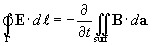
|
From Stokes' theorem, the line integral of the electric field becomes the surface integral of its curl
| (6.5) | 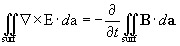
|
Equating the integrands gives the differential form of Faraday's law
| (6.6) | 
|
Since a time-changing magnetic field gives rise to an electric field with curl, we might suspect that a time-changing electric field would produce a magnetic field with curl. Maxwell, in fact, discovered that time-changing electric fields give rise to magnetic fields. If we take the time derivative of Gauss' law
| (6.7) | 
|
and substitute the continuity equation
| (6.8) | 
|
we obtain J = ? ? E/ ? t eliminating ? ?/ ? t. Note, however, that displacement currents result from time-changing electric fields and not charge transport.
Ampere's law is thus...