10.1 Overview

An important part of the life of any physical scientist is comparing theoretical models to data. We now begin three chapters devoted to the nuts and bolts of model fitting. In this chapter, we focus on linear models. ^[1] By a linear model, we mean a model that is linear with respect to the model parameters, not (necessarily) with respect to the indicator variables labeling the data. We will encounter the method of linear least-squares, which is so familiar to most undergraduate science students, but we will see it as a special case in a more general Bayesian treatment.

Examples of linear models:

1. 

   where A ₀, A ₁,... are the linear model parameters, and x _i is the independent (indicator) variable.

2. f _{i , j} = A ₀ + A ₁ x _i + A ₂ y _j + A ₃ x _i y _j

   where A ₀, A ₁,... are the linear model parameters, and x _i, y _j are a pair of independent variables.

3. f _i = A ₁ cos ?t _i + A ₂ sin ?t _i

   where A ₁, A ₂ are the linear model parameters, and ? is a known constant.

4. T _i = Tf _i,

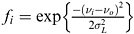
   where T is the linear parameter, and f _i is a Gaussian line shape of the form , and ?