Bayesian Logical Data Analysis for the Physical Sciences

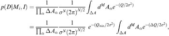
In this section, we are interested in comparing the probabilities of two linear models with different numbers of amplitude parameters. From our treatment of model comparison in Section 3.5, it is clear that the key quantity in model comparison is the evaluation of the global likelihood of a model. Calculation of the global likelihood requires integrating away all of the model parameters from the product of the prior and the likelihood. The integral required to calculate the global likelihood was given earlier as Equation (10.14), which we repeat here:
| (10.122) | |
where we have used Equation (10.59) to expand Q.
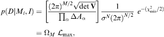
We could do the remaining integral by repeating the process of the preceding Section 10.5.1 for each amplitude: complete the square and integrate, one amplitude at a time. This gets to be very tedious if there are a large number of parameters. A mathematically more elegant approach involves transforming to an orthonormal set of model basis functions. The result is given by
| (10.123) | |
where V is the parameter covariance matrix. The quantity
max is the likelihood for the model at the mode, which is given by
| (10.124) | |
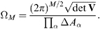
and the Occam factor for the model is
| (10.125) | |
Assigning competing models equal prior probabilities, the posterior probability for a model will be proportional to Equation (10.123). The odds ratio in favor of one model over a competitor is simply given by the ratio of Equation (10.123) for the two models. Suppose model 1 has M