10.8 Frequentist testing and errors

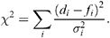
The results in this chapter have been developed from a Bayesian perspective. For comparison purposes, we now introduce a section on model testing and parameter errors from a frequentist perspective. My apologies to those of you who have your Bayesian hat on at this point and can t face the transition again. You can always skip over this section now and return to it if you want to answer question 3(e) in the problems at the end of this chapter. In Section 7.2.1, we discussed the use of the ? ² statistic in hypothesis testing. Once we have determined the best set of model parameters, we can use the ? ² statistic to test if the model is acceptable by attempting to reject the model at some confidence level. From Equation (10.41) we see that ? ² for the fit ^[17] is given by

(10.139)

If the errors are independent, this reduces to the more familiar form:

(10.140)

If the model contains M parameters and there are N data points, then our confidence in rejecting the model is given by the Mathematica command:

Some words of caution are in order on the use of the above for rejecting a hypothesis. First GammaRegularized [( N ? M )/ 2, ? ²/ 2] measures the significance of the test, which equals the area of the ? ² distribution to the right of our measured...