10.4 The posterior is a Gaussian

We have succeeded in finding the most probable model parameters. Now we want to determine the shape of their joint probability distribution with an eye to specifying credible regions for each parameter. We will continue to work with the simple case where all the data errors are assumed to be IID so that p({ A _?} D, I) is given by Equation (10.12),

(10.57)

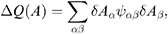
Then maximizing p({ A _?} D, I), corresponds to minimizing Q. Since we ve already taken one derivative of Q (Equation (10.15)), let s see what happens when we take another. Define ?A _? = A _? ? _?. Call the value of Q at the mode Q _min. Recall that the mode is the value that maximizes the probability density. Consider a Taylor series expansion of Q about the Q _min.

(10.58)

The first derivative is zero at the minimum and from Equation (10.8), it is clear there are no higher derivatives than the second. We are now in the position to write Q in a form that explicitly reveals the posterior distribution to be a multivariate Gaussian.

(10.59)

and

(10.60)

Taking another derivative of Equation (10.15) and substituting from Equation (10.31), we get the equation ^[8]

(10.62)

Substituting this into Equation (10.60), we get the equation

(10.63)

where ? is a symmetric matrix. Note: the differential d( ?A _?)...