The Essentials of CAGD

Chapter 7: Working with Polynomial Patches


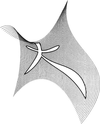
Figure 7.1: A B zier surface trimmed by a ConS. The 2D curve is illustrated in Figure 9.1.

So far, we have covered the basic surface theory. We will now learn to use surfaces for several applications.

7.1 Bicubic Interpolation

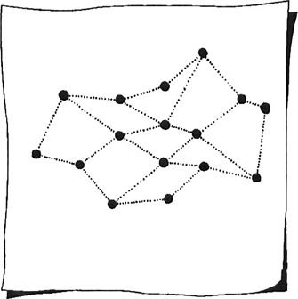
This is one of the simplest surface construction methods. Its uses are limited, but it prepares us for more general approaches. Suppose you are given 16 points p i,j arranged as in Sketch 56 and also a pair of parameter values ( u i, v j) with each of them.


Sketch 56: A 4 4 grid of points.

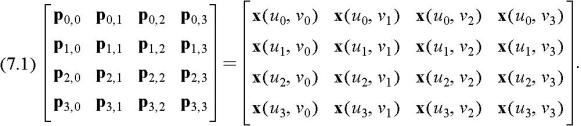
We seek an interpolating bicubic patch x( u, v), such that


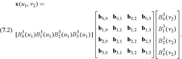
Following the matrix notation of Section 6.3, we may write each x( u i, v j) as a matrix product. We list an example:

x( u 1 v 2) =


We may combine all individual equations for the x( u i, v j) into one matrix equation:


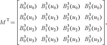
where P is the given matrix of data points as in (7.1) and B is the matrix containing the unknown control points b i,j. The matrix M T contains the values of the Bernstein polynomials at the given parameters:


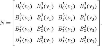
and N is given by


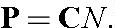
Equation (7.3) is most conveniently decomposed into a sequence of linear systems. First, we define


which reduces (7.3) to


This constitutes four "vector" systems each with four linear equations, all having the...

UNLIMITED FREE
ACCESS
TO THE WORLD'S BEST IDEAS

SUBMIT
Already a GlobalSpec user? Log in.

This is embarrasing...

An error occurred while processing the form. Please try again in a few minutes.

Customize Your GlobalSpec Experience

Category: Commercial Matrix Displays
Finish!
Privacy Policy

This is embarrasing...

An error occurred while processing the form. Please try again in a few minutes.