3.8 Graphical Analysis

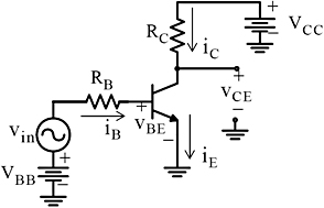
The operation of a simple transistor circuit can also be described graphically. We will use the circuit in Figure 3.42 for our graphical analysis.

Figure 3.42: Circuit showing the variables used in the graphs in Figures 3.43 and 3.44

We start with a plot of i _B versus V _BE to determine the point where the curve

and the equation of the straight line intersect

The equation of (3.41) was obtained with the AC source v _in shorted out. This equation can be expressed as

We recognize (3.42) as the equation of a straight line of the form y=mx+b with slope ?1/R _B. This equation and the curve of equation (3.40) are shown in Figure 3.43.

Figure 3.43: Plot showing the intersection of Equations (3.40) and (3.42)

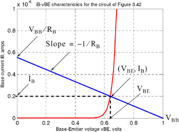
We used the following MATLAB script to plot the curve of equation (3.40).

vBE=0:0.01:1; iR=10<sup^</sup>( 15); beta=100; n=1; VT=27*10^(<span class="unicode">?</span>3);<span class="unicode"> </span>iB=(iR./beta).*exp(vBE./(n.*VT)); plot(vBE,iB); axis([0 1 0 10^(-6)]);<span class="unicode"> </span>xlabel('Base-Emitter voltage vBE, volts'); ylabel('Base current iB, amps');<span class="unicode"> </span>title('iB-vBE characteristics for the circuit of Figure 3.42'); grid 

From Figure 3.43 we obtain the values of V _BE and I _B on the V _BE and i _B axes respectively. Next, we refer to the family of curves of the collector current i _C versus collector-emitter voltage V _CE for different values of i _B as shown in Figure 3.44. where the straight line with slope ?1/R _C is derived from the...