Fundamentals of Signals and Systems

Many physical processes can be represented by, and successfully analyzed with, linear time-invariant (LTI) systems as models. For example, both a DC motor or a liquid mixing tank have constant dynamical behavior (time-invariant) and can be modeled by linear differential equations. Filter circuits designed with operational amplifiers are usually modeled as LTI systems for analysis. LTI models are also extremely useful for design. A process control engineer would typically design a level controller for the mixing tank based on a set of linearized, time-invariant differential equations. DC motors are often used in industrial robots and may be controlled using simple LTI controllers designed using LTI models of the motors and the robot.
It is arguably easier to introduce the concept of convolution in discrete time, which amounts to a sum, rather than in continuous time, where the convolution is an integral. This is why we are starting the discussion of LTI systems in discrete time. We will see that the convolution sum is the mathematical relationship that links the input and output signals in any linear time-invariant discrete-time system. Given an LTI system and an input signal x[ n], the convolution sum will allow us to compute the corresponding output signal y[ n] of the system.
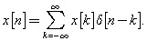
A discrete-time signal x[ n] can be viewed as a linear combination of time-shifted impulses:
| (2.1) | |