Fundamentals of Signals and Systems

In this chapter, we will analyze the behavior of stable continuous-time linear time-invariant (LTI) systems by looking at both the time-domain and the frequency-domain points of view. We will see how to get a feel for the frequency response of a system by looking at its transfer function in pole-zero form. We will also introduce the Bode plot, which is a representation of the frequency response of a system that can be sketched by hand.
A standing assumption here is that the causal LTI system is stable. This means that all the poles of the transfer function lie in the open left half-plane. On the other hand, the zeros do not have this restriction.
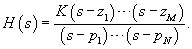
We want to be able to characterize qualitatively the system's frequency response from the knowledge of the poles and zeros of the transfer function. Consider a transfer function written in its pole-zero form:
| (8.1) | |
When we let s =j ?, each first-order pole and zero factor can be seen as a vector whose origin is at the pole (zero) and whose endpoint is at j ?. For a fixed frequency ?, each of these vectors adds a phase contribution and a magnitude factor to the overall frequency response. Let us illustrate this by means of two examples.
A stable first-order system with transfer...