Fundamentals of Signals and Systems

The Laplace transform is a powerful tool to solve linear time-invariant (LTI) differential equations. We have used the Fourier transform for the same purpose, but the Laplace transform, whether bilateral or unilateral, is applicable in more cases, for example, to unstable systems or unbounded signals.
We have seen that the transfer function of an LTI system is the Laplace transform of its impulse response. For a differential LTI system, the transfer function can be readily written by inspecting the differential equation, just like its frequency response can be obtained by inspection.
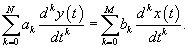
Consider the general form of an LTI differential system:
| (7.1) | |
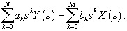
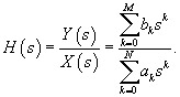
We use the differentiation and linearity properties of the Laplace transform to obtain the transfer function H( s) = Y( s)/ X( s):
| (7.2) | |
| (7.3) | |
Note that we have not specified a region of convergence (ROC) yet. This means that differential Equation 7.1 can have many different impulse responses; that is, it is not a complete specification of the LTI system. If we know that the differential system is causal, then the ROC is the open right half-plane to the right of the rightmost pole in the s-plane. The impulse response is then uniquely defined.
Let n( s) :=
b ks k be the numerator polynomial of the transfer function H(