Fundamentals of Signals and Systems

Chapter 10: State Models of Continuous-Time LTI Systems

LECTURE 33: STATE MODELS OF CONTINUOUS-TIME LTI SYSTEMS

In Chapter 3 we studied an important class of continuous-time linear time-invariant (LTI) systems defined by linear, causal constant-coefficient differential equations. For a system described by an N th-order differential equation, it is always possible to find a set of N first-order differential equations and an output equation describing the same input-output relationship. These N first-order differential equations are called the state equations of the system. The states are the N variables seen as outputs of the state equations.

The concept of state is directly applicable to certain types of engineering systems such as linear circuits and mechanical systems. The state variables in a circuit are the capacitor charges (or equivalently the voltages since q = Cv) and the inductor currents. In a mechanical system, the state variables are generally the position and velocity of a body.

Before we move on, an important word on notation: for state-space systems, the input signal is conventionally written as u( t) (not to be confused with the unit step) instead of x( t), as the latter is used for the vector of state variables. Hence, in this chapter we will use q( t) to denote the unit step signal.

STATE MODELS OF CONTINUOUS-TIME LTI DIFFERENTIAL SYSTEMS

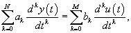
Consider the general N th-order causal linear constant-coefficient differential equation with M ? N:

(10.1)

which can be expanded to

(10.2)

UNLIMITED FREE
ACCESS
TO THE WORLD'S BEST IDEAS

SUBMIT
Already a GlobalSpec user? Log in.

This is embarrasing...

An error occurred while processing the form. Please try again in a few minutes.

Customize Your GlobalSpec Experience

Category: Flow Switches
Finish!
Privacy Policy

This is embarrasing...

An error occurred while processing the form. Please try again in a few minutes.