20.9 Discrete Time Integration with Variable Amplitude Input

In Chapter 2, Exercise 12, we showed that when the input signal is a pulse, a Discrete Forward Euler Integrator and a Discrete Trapezoidal Integrator will produce the same result. In this example, we will use an input that varies in amplitude during a sample period. This is illustrated with the model in Figure 20.87.

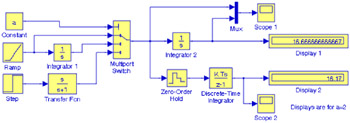Figure 20.87: Model for Discrete Time Integration with variable amplitude input

For the model in Figure 20.71, we have used the following settings:

Simulation Configuration Parameters

Solver: Ode4 (Runge-Kutta)

Type: Fixed Step Size

Fixed Step Size: 0.01

Start Time: 0

Stop Time: 10

Ramp block

Slope: 0.1

Step block

Final Value: 5

Transfer Function block

Numerator: [1 0]

Denominator: [1 1]

Multiport Switch block

Number of inputs: 3

Zero Order Hold block

Sample time: 0.2

Discrete Time Integrator block

Integrator method: User's choice

Sample time: -1 (Inherent from input)

Display 1 and Display 2 blocks

Format: Long

In MATLAB command prompt enter:

a = 1 for testing a discrete integrator with a ramp input signal

a = 2 for testing a discrete integrator with a parabolic input signal - chosen for this model

a = 3 for testing a discrete integrator with an exponentially decaying signal

All other unlisted parameters are left in their default states

Upon execution of the simulation command, the waveforms displayed by the Scope 1 and Scope 2 blocks are shown in Figures 20.72 and...