Phase-Locked Loops for Wireless Communications: Digital, Analog and Optical Implementations, Second Edition
In Chapter 2, we presented the basic configurations for phase-locked loops. We would like to present the performance and dynamics of phase-locked loops next, but at this point, we don't have enough theory to design the loops. Recall in Chapter 2, we mentioned terms such as damping factors, and with the third-order loop, unity gain crossover. So before we can discuss the true performance of phase-locked loops, we need to build expand the theoretical foundation.
In Chapter 2, we developed the transfer functions H o( s) and H e( s). H o( s) represents the transfer function for the output of the VCO. H e( s) is the transfer function relative to the output of the phase detector. These transfer functions permit us to write the outputs of the phase-locked loop as
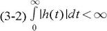
Assuming the input ? i( t), is bounded, ( ? i( t)< ?), we are interested in knowing whether the output, ? o( t), is also bounded. From linear systems theory, a linear system is stable if and only if the integral of the absolute value of the impulse function is finite [1]. In other words,
Recall the Ho(s) for the second order, type-2 loop (the active filter configuration) is
The poles of a transfer function correspond to the roots of the denominator's polynomial equation. In other words, for Equation 3-3, the solutions for s 2 = 2