Phase-Locked Loops for Wireless Communications: Digital, Analog and Optical Implementations, Second Edition
To begin our study of the digital phase-locked loop, we will begin by translating the analog loop equations of Chapters 2 and 3 to the discrete-time domain. A reader may question this approach, so we quote Oppenheim and Schafer's explanation of translating analog filters to the digital domain [1].
The art of analog filter design is highly advanced and, since useful results can be achieved, it is advantageous to utilize the design procedures already developed for analog filters.
Many useful analog design methods have relatively simple closed-form design formulas. Therefore, digital filter design methods based on such analog design formulas are rather simple to implement.
In many applications it is of interest to use a digital filter to simulate the performance of an analog linear time-invariant filter.
We believe the same statements are valid for converting analog phase-locked loop designs to the digital domain.
We will show how the analog configurations of Chapter 2 can be transformed directly into corresponding discrete versions. There are different transformations possible, the most noteworthy being the backward difference and bilinear transformations. The time-domain equations will be emphasized similar to our development of the analog loops.
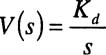
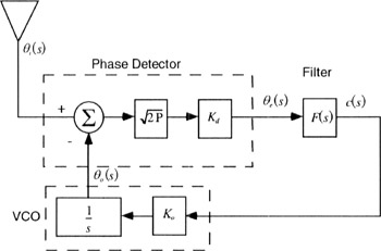
Figure 7.1 reviews the block diagram of an analog phase-locked loop. The presence of the VCO's transfer function of
in the analog phase-locked loop yields a time-domain solution in the form of a differential equation. We repeat here the differential equation for the first-order analog phase-locked loop.