Ordinary Differential Equations in Theory and Practice

7. Infectious Diseases II

7. Infectious Diseases II

The epidemic model in 6 is suitable for infectious diseases with a uniform spatial distribution. Here we study the effect when this distribution is nonhomogeneous. One may think of diseases penetrating a population via contacts between individuals. Examples are influenza, rabies, pest, and Aids. For convenience, the following assumptions are being made:

  • The incubation time is negligibly short.

  • The pathogens can only survive and reproduce themselves while residing in infected individuals.

  • Every infected individual recovers or dies after some time. Recovered individuals become immune.

The model has to describe the time and space dependence of:

y 1( t, x):

concentration of individuals not yet infected and thus susceptible individuals,

y 2( t, x):

concentration of infected individuals.

In fact a third class y 3 plays a r le in the model, namely the class of recovered and thus immune individuals. Because of the relation y 1+ y 2+ y 3=1 it is not necessary to introduce separate formulae for y 3.

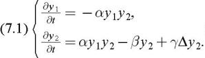
The concentrations are taken with respect to the population density y , averaged over the region and time period under consideration. In view of the considerations above, we describe the interactions between the two classes y 1 and y 2 by the following equations:


The rationale of the different terms is as follows:

  • ? ?y 1 y 2 with rate of infection ?>

UNLIMITED FREE
ACCESS
TO THE WORLD'S BEST IDEAS

SUBMIT
Already a GlobalSpec user? Log in.

This is embarrasing...

An error occurred while processing the form. Please try again in a few minutes.

Customize Your GlobalSpec Experience

Category: Infrared Thermometers
Finish!
Privacy Policy

This is embarrasing...

An error occurred while processing the form. Please try again in a few minutes.