Feedback linearization has been studied extensively in the nonlinear systems literature (see, for example, [121,134,159,185]). In this text, we cover only some of the basic background to help the reader understand some of the techniques that will be used in Chapters 6 and 7 in the context of adaptive approximation based control. In this subsection, we present the concept of input-output linearization.

Consider the single-input single-output (SISO) nonlinear system

where u ∈ ¹, y ∈ ¹, x ∈ ⁿand ƒ, g and h are sufficiently smooth in a domain D ⊂ ⁿ. The time derivative of y = h(x) is given by

If for any x ∈ D₀ then the nonlinear system is said to have relative degree one on D₀. Intuitively, this implies that the control variable u appears explicitly in the differential equation for the first derivative of the output y; i.e., the input and output are separated by a single integrator. If (i.e., u does not directly affect ), then we keep on differentiating the output until u appears explicitly. In order to define the second, third (and so on) derivatives, it is convenient to define the concept of a Lie derivative, which is used in advanced calculus.

The notation for the Lie derivative of h with respect to ƒ is defined as

This notation is convenient for dealing with repeated derivatives, as shown below:

Based on the definition of the Lie derivative, if

we keep on taking derivatives until , which implies that u first appears explicitly in the equation for y^(r), the r-th derivative of the output.

The nonlinear system (5.33)-(5.34) is said to have a relative degree r in a region D₀ ⊂ D if the following conditions are satisfied for any x ∈ D₀:

If a system has relative degree r, then

Hence, the system is input-output linearizable, since the state feedback control

gives the following linear input-output mapping:

This is simply a chain of r integrators, which can be easily controlled by an appropriate selection of v. However, unless r = n, there are more states in the system that are not affected by the control input u. The dynamics of this set of (n – r) states will define the so-called zero dynamics of the system, which are discussed below.

Using differential geometric tools, it can be shown that for a system with relative degree r there exists a diffeomorphism z = T(x) that would transform the nonlinear system (5.33)-(5.34) into the input-output linearizable canonical form

where z = [n^T ζ^T]^T, with n ∈ ^{n – r}, ζ ∈ ^r, and (A₀, B₀, C₀) is a canonical form representation of a system consisting of r integrators in series:

The diffeomorphism z = T(x), with T(0) = 0, which transforms the nonlinear system (5.33)-(5.34) into the canonical form (5.36)-(5.38) is characterized by

The transformed system described by (5.36)-(5.38) is said to be in normal form. Basically, the nonlinear system is decomposed in two parts, the ζ-dynamics, which can be linearized by feedback, and the n variables, which characterize the internal dynamics of the system. The ζ-dynamics can be linearized and controlled by utilizing a feedback controller of the form

where v can be chosen to set the convergence rate of the ζ-dynamics or to achieve reference input tracking. The feedback linearizing control functions α₀ and β₀ are computable based on the Lie derivatives obtained by differentiating the output variable:

The zero dynamics are obtained by setting ζ = 0 in the n-dynamics:

The nonlinear system is said to be minimum phase if the zero dynamics described by (5.40) have an asymptotically stable equilibrium point in D.

The concepts of relative degree, coordinate decomposition into the n and ζ dynamics, minimum phase, zero dynamics, etc. all have their corresponding equivalents for linear systems. Of course, for linear systems we have the concept of a transfer function which characterizes both the stability of the input-output system (by the location of the roots of the denominator polynomial - the poles), as well as the stability of the internal dynamics, which are given by the roots of the numerator polynomial - the zeros.

Consider the n-th order linear system described by the transfer function

where r is the relative degree of the system; i.e., the difference between the order of the denominator and the order of the numerator. A state model (non-unique) for the system is given by

where we are assuming that r ≥ 1, thus the D matrix is zero. By taking the first time derivative of the output y(t), we obtain

If r = 1 (relative degree 1) then CB ≠ 0. On the other hand, if CB = 0, then the relative degree is larger than 1 so we continue to take time derivatives of the output. Following this procedure it can be shown that for linear systems with relative degree r,

and the r-th derivative of v(t) satisfies

Moreover, the dynamics of the linear system can be broken up into two components as follows: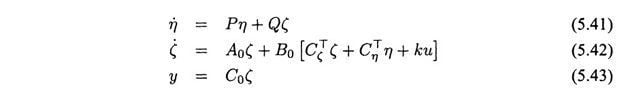

where n ∈ ^{n – r}, ζ ∈ ^r, the triple (A₀, B₀, C₀) is a canonical form representation of r integrators, as described by (5.39), P and Q are matrices of appropriate dimension, C_ζis a vector of dimension r, and C_n is a vector of dimension (n – r).

The reader will note that (5.41)-(5.43) is a linear special case of the normal form described by (5.36)-(5.38). The zero dynamics of the linear system, as defined earlier for the general normal form of nonlinear systems, are obtained by setting ζ = 0 in (5.41). This yields

The stability of the zero dynamics are determined by the eigenvalues of P. The model is said to be minimum phase if all the eigenvalues are in the left open-half complex plane. It is important to note that the eigenvalues of P turn out to be the same as the roots of the numerator of the transfer function H(s). This justifies the use of the term zero dynamics for nonlinear systems.

One question that may be raised in obtaining the normal form for nonlinear systems is whether any system can be put into the canonical normal form. In general, the answer is negative since for some systems the relative degree is undefined. This may happen, for example, if , where k₀ is a scalar constant. This implies that is zero for x₁= 0 but it is nonzero in any neighborhood of x₁= 0.

Next, we consider the tracking control design for input-output feedback linearizable systems. We assume that the control objective is for y(t) to track a desired signal y_d (t). Let e(t) = y(t) - y_d (t) be the tracking error. Starting from the normal form (5.36)-(5.38) we design the feedback control law

where v is selected as follows:

The control law (5.45)-(5.46) results in the linear error dynamics

Therefore, by appropriately selecting the coefficients {k₀, k₁, ... k_{r – 2}, k_{r – 1}}the roots of the characteristic equation

can be arbitrarily assigned. This implies that the tracking error can be made to converge to zero asymptotically (exponentially fast).

From the normal form (5.36)-(5.38), we note that the above control design has taken care only of the ζ variables. The designer also needs to be assured that the internal dynamics, , remain bounded when the control law is designed for the ζ-dynamics. This issue is addressed next.

Let

As shown by Isidori [121], it we assume that is bounded for all t ≥ 0 and the solution of

is well defined, bounded, and uniformly asymptotically stable, then using the control law (5.45)-(5.46) guarantees that the whole state remains bounded and the tracking error e(t) converges to zero exponentially fast.

In the special case of regulation to the origin; i.e., y_d (t) – 0 for all t > 0, then it is required that the zero dynamics

are asymptotically stable in order to ensure that the overall system states remain bounded and the tracking error converges to zero.

In summary, we note that for input-output linearizable systems there are two components to be taken care of:

• the ζ-dynamics, which can be linearized by the control variable u, and
  
  
• the -dynamics, referred to as internal dynamics, which are rendered unobservable by the u defined in (5.35), but which need to have some stability properties (minimum phase) in order to allow stable control of the overall system.

■ EXAMPLE 5.5

Consider the flexible manipulator model of Example 5.4, whose state representation is given by

First consider the case where the output y = x₁. In this case the diffeomorphism z = T(x) given by (5.30) transforms the system into the normal form since

is already in the form described by (5.36)-(5.36). The relative degree is 4, which is the same as the order of the nonlinear system; hence, there are no internal dynamics.

Next, consider the case where the output is given by y = x₃. By taking time derivatives of y(t), we note that the control input u appears in the second derivative:

Therefore, in this case the relative degree is 2. The input-output feedback linearizing controller designed for tracking the signal y_dis

for λ₁, λ₂ > 0. This controller renders x₁ and x₂ unobservable from y. The system is already in normal form, without any transformation, since the first two variables x₁, x₂, are the-dynamics which characterize the internal dynamics of the system. The last two variables x₃, x₄, are the ζ-dynamics, which are in the canonical form. The zero dynamics are obtained from the variables by setting x₃ and x₄ to zero. Therefore the zero dynamics are given by

■ EXAMPLE 5.6

Consider the system

where α is a constant. The objective is to transform the system into normal form and to design a feedback linearizing controller. By taking the first two time derivatives of y(t) we obtain

Therefore, the relative degree of the system is 2. By using the diffeomorphism

we can convert the system into the normal form:

By selecting the feedback control law

The zero dynamics are obtained by setting ζ₁, ζ₂ to zero in the -dynamics, which yields

Therefore, the zero dynamics are globally asymptotically stable, which implies that the system is minimum phase. This can be seen from the fact that the solutions of the zero dynamics with initial conditions (t₀) = ₀ are given by

The last example illustrates one of the key drawbacks of feedback linearization: it depends on exact cancellation of nonlinear functions. If one of the functions is uncertain then cancellation is not possible. This is one of the motivations for adaptive approximation based control.

Another possible difficulty with feedback linearization is that not all systems can be transformed to a linearizable form. The next section presents another technique, referred to as backstepping, which can be applied to a class of systems which may not be feedback linearizable.