In parallel with developments in adaptive nonlinear control, there has been a tremendous amount of activity in neural control and adaptive fuzzy approaches. In these studies, neural networks or fuzzy approximators are used to approximate unknown nonlinearities. The input/output response of the approximator is modified by adjusting the values of certain parameters, usually referred to as weights. From a mathematical control perspective, neural networks and fuzzy approximators represent just two classes of function approximators. Polynomials, splines, radial basis functions, and wavelets are examples of other function approximators that can be used and have been used in a similar setting. We refer to such approximation models with adaptivity features as adaptive approximators, and control methodologies that are based on them as adaptive approximation based control. Adaptive approximation based control encompasses a variety of methods that appear in the literature: intelligent control, neural control, adaptive fuzzy control, memory-based control, knowledge-based control, adaptive nonlinear control, and adaptive linear control. |
 During the last few years there have been significant developments in the control of highly uncertain, nonlinear dynamical systems. For systems with parametric uncertainty, adaptive nonlinear control has evolved as a powerful methodology leading to global stability and tracking results for a class of nonlinear systems. Advances in geometric nonlinear control theory, in conjunction with the development and refinement of new techniques, such as the backstepping procedure and tuning functions, have brought about the design of control systems with proven stability properties. In addition, there has been a lot of research activity on robust nonlinear control design methods, such as sliding mode control, Lyapunov redesign method, nonlinear damping, and adaptive bounding control. These techniques are based on the assumption that the uncertainty in the nonlinear functions is within some known, or partially known, bounding functions.
Chapter 5.4.3 - Lyapunov Redesign Method
Consider a nonlinear system described by  where x ∈  where ƒ0 and G0 characterize the known nominal plant, and ƒ*, G* represent the uncertainty. Later we will assume that the unknown portion satisfies a certain bounding condition. Moreover, we assume that the uncertainty satisfies a so-called matching condition:  The matching condition implies that the uncertainty terms appear in the same equations as the control inputs u, and as a result they can be handled by the controller. By substituting (5.88)-(5.89) and (5.90)-(5.91) in (5.87) we obtain  where comprises all the uncertainty terms, and is given by  The Lyapunov redesign method addresses the following problem: suppose that the equilibrium of the nominal model Next, we consider the details of the Lyapunov redesign method, which is thoroughly presented for a more general case in [134]. We assume that there exists a control law u = p0(x)such that x = 0 is a uniformly asymptotically stable equilibrium point of the closed-loop nominal system  We also assume that we know a Lyapunov function V0(x) that satisfies  where α1, α2, α3: The uncertainty term is assumed to satisfy the bound  where the bounding function Now, we will proceed to the design of the corrective "control component" p*(x) such that u = p0 + p* stabilizes the class of systems described by (5.92) and satisfying (5.95). The corrective control term is designed based on a technique following the nominal Lyapunov function V0, which justifies the name Lyapunov redesign method. Consider the same Lyapunov function V0 that guarantees the asymptotic stability of the nominal closed-loop system, but now consider the time derivative of V0 along the solutions of the full system (5.92). We have  where  which is a known function. By taking bounds we obtain  The second term of the right-hand side of (5.97) can be made zero if  Each component of the corrective control vector p*(x) is selected to be of the form p*(x) = By substituting (5.98) in (5.97) we obtain the desired "stability" property  which implies that the closed-loop system is asymptotically stable. The augmented control law u = p0(x) + p*(x) is discontinuous since each element This can be achieved by replacing (5.98) with  where ε > 0 is a small design constant. Note that as ε approaches zero, the tanh By substituting (5.99) in (5.97) we obtain  Using Lemma A.5.1 (see p. 397),  where = 0.2785. Since α3 is a class The following example illustrates the use of the Lyapunov redesign method. ■ EXAMPLE 5.9 Consider the nonlinear system  where is unknown but is known to satisfy the inequality  for some known bound The first step is to design the nominal control law u = p0(x) for the case of = 0. This can be accomplished by feedback linearization (note that it can also be accomplished by the backstepping method). Consider the change of coordinates z = T(x) where  The dynamics in the z-coordinates are described by  where z(z) = (x)x=T -1(z). A stabilizing nominal controller is given by  A nominal Lyapunov function associated with the above nominal controller is given by  whose time derivative is given by  Since by eqn. (5.96) (z) = 2(z1 + z2), the corrective feedback control law obtained using the Lyapunov redesign method is given by  where 
|
 nis the state and u ∈
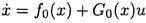 can be made uniformly asymptotically stable by using a feedback control law u = p0(x). The objective is to design a corrective control function p*(x) such that the augmented control law u = p0(x) + p*(x) is able to stabilize the system (5.92) subject to the uncertainty (x, u) being bounded by a known function.
 is assumed to be known a priori or available for measurement.
 can be of large magnitude if the uncertainty bound
  is large. As discussed earlier, discontinuities in the control law can cause chattering, therefore it is desirable to smooth the discontinuity and at the same time retain to some degree the nice stability properties of the original discontinuous control law.
 function converges to the discontinuous sgn( i) function.
  and for any r > 0, there exists an ε (sufficiently small), such that
  for x outside a region Dε = {x V(x) ≤ r}. Therefore, the trajectory is convergent to the invariant set Dε.
 . This second-order model represents a jet engine compression system with no-stall [139], which is based on the Galerkin approximation or the nonlinear PDE model [176]. The state x1 corresponds to the mass flow and x2 is the pressure rise.
 is the assumed bound on . The above control law can be made continuous using the following approximation