In the previous two subsections we have described the procedure for linearizing around an operating point x_eor around a trajectory x*(t). As discussed, a key limitation of the small-signal linearization approach is the fact that the linear model is accurate only in a neighborhood around the operating point x_eor the nominal trajectory x*. Consequently, the linear control law that is designed based on the linear model is, in general, effective only if the system state remains in that same neighborhood. In this subsection we introduce the gain scheduling control approach, which is based on small-signal linearization around multiple operating points. For each linear model we design a feedback controller, thus creating a family of feedback control laws, each applicable in the neighborhood of a specific operating point. The family of feedback controllers can be combined into a single control whose parameters are changed by a scheduling scheme based on the trajectory or some other scheduling variables.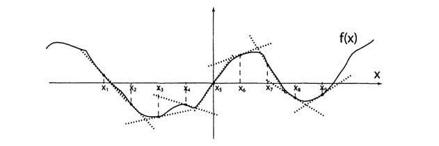

Figure 5.3: Diagram to illustrate the gain scheduling approach, which is based on the linearization around multiple operating points {x₁, x₂ ... x₉}. The multiple linear models constitute an example of approximating a nonlinear system.

Consider again the nonlinear system (5.1), where in this case we linearize the system into N linear models

where z = x – x₁ for each i. Each linear model parameterized by (A_i, B_i) is valid around an operating point point x₁. This is illustrated in Figure 5.3, where the nonlinear function ƒ(x) is linearized around nine operating points {x₁, x₂ ... x₉}. For each linear model we design a control law based on the control objective associated with a particular operation point. Suppose that the control law u = K_iz corresponds to the linear model . A key element of the gain scheduling approach is the design of a scheduler for switching between the various control laws parameterized by {K₁, K₂ ... K_N}. Typically, transitions between different operating points are handled by interpolation methods. The gain scheduler can be viewed as a look-up table with the appropriate logic for selecting a suitable controller gain K_ibased on identifying the corresponding operating point x₁.

Intuitively, we note that if the region of attraction associated with each linearization is larger than the scheduled operating region corresponding to each operating point, then the resulting gain scheduling control scheme will be stable. However, special care needs to be taken since the resulting controller is time-varying, hence the stability analysis needs to be treated as a time-varying system. A formal stability analysis for gain scheduling is beyond the scope of this text (see the work of Shamma and Athans [242, 243]).

Despite the derivation of some stability results under certain conditions, gain scheduling is still considered to some degree an ad hoc control method. However, it has been used in several application examples, especially in flight control [118, 161, 183, 256, 257, 258]. The gain scheduling approach has also been utilized in other applications such as in process control and automotive applications [11, 113, 126].

One of the key limitations of gain scheduling is that the controller parameters are pre-computed offline for each operating condition. Hence, during operation the controller is fixed, even though the linear control gains are changing as the operating conditions change. In the presence of modeling errors or changes in the system dynamics, the gain scheduling controller may result in deterioration of the performance since the method does not provide any learning capability to correct – during operation – any inaccurate schedules. Another possible drawback of the gain scheduling approach is that it requires considerable offline effort to derive a reliable gain schedule for each possible situation that the plant will encounter.

The gain scheduling approach can be conveniently viewed as a special case of the adaptive approximation approach developed in this text. A local linear model is an example case of a local approximation function. For example, the linear functions in Figure 5.3 can be replaced by other approximation functions. Typically, the adaptive approximation based techniques developed in this book consist of approximation functions with at least some overlap between, which intuitively can be viewed as a way to obtain a smoother approximation from one operating position (or from one node) to another.

One of the key differences between the standard gain scheduling technique and the adaptive approximation based control approach is the ability of the latter to adjust certain parameters (weights) during operation. Unlike gain scheduling, adaptive approximation is designed around the principle of "learning" and thus reduces the amount of modeling effort that needs to be applied offline. Moreover, it allows the control scheme to deal with unexpected changes in plant dynamics due to faults or severe disturbances.