In parallel with developments in adaptive nonlinear control, there has been a tremendous amount of activity in neural control and adaptive fuzzy approaches. In these studies, neural networks or fuzzy approximators are used to approximate unknown nonlinearities. The input/output response of the approximator is modified by adjusting the values of certain parameters, usually referred to as weights. From a mathematical control perspective, neural networks and fuzzy approximators represent just two classes of function approximators. Polynomials, splines, radial basis functions, and wavelets are examples of other function approximators that can be used and have been used in a similar setting. We refer to such approximation models with adaptivity features as adaptive approximators, and control methodologies that are based on them as adaptive approximation based control. Adaptive approximation based control encompasses a variety of methods that appear in the literature: intelligent control, neural control, adaptive fuzzy control, memory-based control, knowledge-based control, adaptive nonlinear control, and adaptive linear control. |
 During the last few years there have been significant developments in the control of highly uncertain, nonlinear dynamical systems. For systems with parametric uncertainty, adaptive nonlinear control has evolved as a powerful methodology leading to global stability and tracking results for a class of nonlinear systems. Advances in geometric nonlinear control theory, in conjunction with the development and refinement of new techniques, such as the backstepping procedure and tuning functions, have brought about the design of control systems with proven stability properties. In addition, there has been a lot of research activity on robust nonlinear control design methods, such as sliding mode control, Lyapunov redesign method, nonlinear damping, and adaptive bounding control. These techniques are based on the assumption that the uncertainty in the nonlinear functions is within some known, or partially known, bounding functions.
Chapter 5.5 - Adaptive Nonlinear Control
Adaptive control deals with systems where some of the parameters are unknown or slowly time-varying. The basic idea behind adaptive control is to estimate the unknown parameters online using parameter estimation methods (such as those presented in Chapter 4), and then to use the estimated parameters, in place of the unknown ones, in the feedback control law. Most of the research in adaptive control has been developed for linear models, even though in the last decade or so there has been a lot of activity on adaptive nonlinear control as well. Even in the case of adaptive control applied to linear systems, the resulting control law is nonlinear. This is due to the parameter update laws, which render the feedback controller nonlinear. There are two strategies for combining the control law and the parameter estimation algorithm. In the first strategy, referred to as indirect adaptive control, the parameter estimation algorithm is used to estimate the unknown parameters of the plant. Based on these parameter estimates, the control law is computed by treating the estimates as if they were the true parameters, based on the certainty equivalence principle [11]. In the second strategy, referred to as direct adaptive control, the parameter estimator is used to estimate directly the unknown controller parameters. It is interesting to note the similarities and difference between so called robust control laws and adaptive control laws. The robust approaches, which were discussed in Section 5.4, treat the uncertainty as an unknown box where the only information available are some bounds. The robust control law is obtained based on these bounds, and in fact is designed to stabilizes the system for any uncertainty within the assumed bounds. As a result, the robust control law tends to be conservative and it may lead to large control input signals or control saturation. On the other hand, adaptive control assumes a special structure for the uncertainty where the nonlinearities are known but the parameters are unknown. In contrast to robust control, in adaptive control the objective is to try to estimate the uncertain (or time-varying) parameters to reduce the level of uncertainty. In the next chapter, we will start investigating the adaptive approximation control approach where the uncertainty also includes nonlinearities that are estimated online. Hence, adaptive approximation based control can be viewed as an expansion of the adaptive control methodology where instead of having simply unknown parameters we have unknown nonlinearities. Adaptive control is a well-established methodology in the design of feedback control systems. The first practical attempts to design adaptive feedback control systems go back as far as the 1950s, in connection with the design of autopilots [295]. Stability analysis of adaptive control for linear systems started in the mid-1960s [196] and culminated in 1980 with the complete stability proof for linear systems [69, 177, 180]. The first stability results assumed that the only uncertainty in the system was due to unknown parameters; i.e., no disturbances, measurement noise, nor any other form of uncertainty. In the 1980s, adaptive control research focused on robust adaptive control for linear systems, which dealt with modifications to the adaptive algorithms and the control law in order to address some types of uncertainties [119]. In the 1990s, most of the effort in adaptive control focused on adaptive control of nonlinear systems with some elegant results [139]. To illustrate the use of the adaptive control methodology we consider below two examples of adaptive nonlinear control. ■ EXAMPLE 5.11 In this example we consider the feedback linearization problem of Section 5.2 with unknown parameters. Consider the n-th order model  where θ1, θ2, θ3 are unknown, constant parameters and ƒ1 andƒ2 are known functions. The objective is to design an adaptive controller such that y(t) = x1(t) tracks a desired signal yd (t). Let e = y – ydbe the tracking error. If θ1, θ2, θ3were known and θ3 ≠ 0 then the control law  would result in the following tracking error dynamics:  The coefficients {λ1, λ2, ... λn-1} would be selected such that the characteristic polynomial  has all its roots in the left-halt complex plane. Since θ1, θ2, θ3 are unknown, we replace them in the control law by their corresponding estimates  which yields the following tracking error dynamics  where  where A0, B0 is the canonical form pair given by 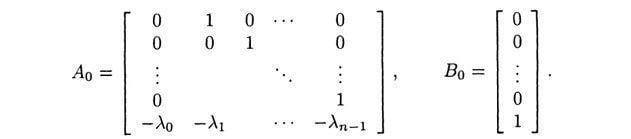 Since A0is a stability matrix, there exists a positive definite matrix P such that  We choose the Lyapunov function  whose time derivative along the solution of the tracking error dynamics is given by 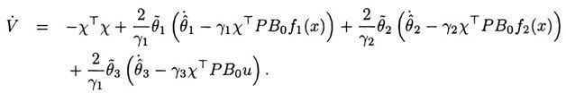 Therefore, we select the adaptive laws as follows:  Clearly, this results in 
■ EXAMPLE 5.12 In this example we consider the backstepping control procedure of Section 5.3 for the case where there is an unknown parameter. Consider the second-order system  where θ is an unknown parameter and ƒ is a known function. The parameter estimate for θ is defined as We define the change of coordinates  where α is defined as
The dynamics of the new coordinates z1, z2 are given by
where
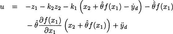
where the term in the second line cannot be computed. Therefore, the feedback control law is selected as follows:
Where k2 > 0 is a design constant. The resulting closed-loop z dynamics are given by
Now, consider the time derivative of the Lyapunov function candidate  where γ > 0 is the adaptive gain. We have 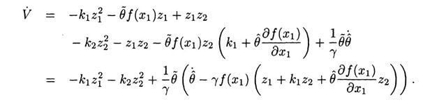 Based on the above derivative of the Lyapunov function, we select the update law for  Hence, 
|
 , where it is assumed for the time being that
  for all t ≥ 0. The adaptive control law is given by
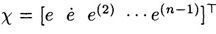 then the tracking error dynamics can be written as
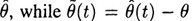 is the parameter estimation error. The objective is to design an adaptive nonlinear tracking controller such that y = x1 tracks a desired signal yd(t).

 denotes the time derivative of α; which can be computed as follows:

 as follows:
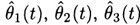
 are uniformly bounded and z1, z2both converge to zero.