In parallel with developments in adaptive nonlinear control, there has been a tremendous amount of activity in neural control and adaptive fuzzy approaches. In these studies, neural networks or fuzzy approximators are used to approximate unknown nonlinearities. The input/output response of the approximator is modified by adjusting the values of certain parameters, usually referred to as weights. From a mathematical control perspective, neural networks and fuzzy approximators represent just two classes of function approximators. Polynomials, splines, radial basis functions, and wavelets are examples of other function approximators that can be used and have been used in a similar setting. We refer to such approximation models with adaptivity features as adaptive approximators, and control methodologies that are based on them as adaptive approximation based control. Adaptive approximation based control encompasses a variety of methods that appear in the literature: intelligent control, neural control, adaptive fuzzy control, memory-based control, knowledge-based control, adaptive nonlinear control, and adaptive linear control. |
 During the last few years there have been significant developments in the control of highly uncertain, nonlinear dynamical systems. For systems with parametric uncertainty, adaptive nonlinear control has evolved as a powerful methodology leading to global stability and tracking results for a class of nonlinear systems. Advances in geometric nonlinear control theory, in conjunction with the development and refinement of new techniques, such as the backstepping procedure and tuning functions, have brought about the design of control systems with proven stability properties. In addition, there has been a lot of research activity on robust nonlinear control design methods, such as sliding mode control, Lyapunov redesign method, nonlinear damping, and adaptive bounding control. These techniques are based on the assumption that the uncertainty in the nonlinear functions is within some known, or partially known, bounding functions.
Chapter 5.3.1 - Second Order System
To illustrate the concept of backstepping, or integrator backstepping, we start with a simple second-order system:  where (x1, x2) ∈ The key idea behind the backstepping procedure is that the tracking problem would be solved if the control input u could force x2(t) to satisfy  with k1 > 0. In this case  By adding and subtracting  If we let z1 = x1– ydthen z1 satisfies  Now, consider a coordinate transformation  whose derivative is given by
where
With this change of variables, we have rewritten the original system (5.48)-(5.49) as the tracking error dynamics:  The main, and key difference, between the original system (5.48)-(5.49) and the modified system (5.51)-(5.52) is that the modified system has an equilibrium at the origin and the z1 dynamics of that equilibrium are asymptotically stable when z2 = 0 and v = 0. Now consider the Lyapunov function  whose time derivative along the solutions of (5.51)-(5.52) is given by  If we select the modified control input as  which shows that the equilibrium point (z1, z2) = (0,0) of the closed-loop tracking error dynamics is globally asymptotically stable. From the definition of v we conclude (by combining (5.50) and (5.53)) that the feedback control law u given by  results in a globally asymptotically stable origin for the (z1, z2) system that ensures perfect tracking of yd by x1, assuming of course, that g(x1) is bounded away from zero for all x1 ∈ Some remarks:
|
 2is the state, g(x1) ≠0 for x1 in some domain D that defines the operating envelope, and u ∈
  satisfies
 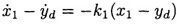 , which implies that x1(t) converses to yd(t). This is equivalent to treating x2 as a virtual control input for the x1 subsystem. Therefore, we introduce the virtual control variable
  , which is defined as
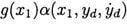 in (5.48) we obtain