In parallel with developments in adaptive nonlinear control, there has been a tremendous amount of activity in neural control and adaptive fuzzy approaches. In these studies, neural networks or fuzzy approximators are used to approximate unknown nonlinearities. The input/output response of the approximator is modified by adjusting the values of certain parameters, usually referred to as weights. From a mathematical control perspective, neural networks and fuzzy approximators represent just two classes of function approximators. Polynomials, splines, radial basis functions, and wavelets are examples of other function approximators that can be used and have been used in a similar setting. We refer to such approximation models with adaptivity features as adaptive approximators, and control methodologies that are based on them as adaptive approximation based control. Adaptive approximation based control encompasses a variety of methods that appear in the literature: intelligent control, neural control, adaptive fuzzy control, memory-based control, knowledge-based control, adaptive nonlinear control, and adaptive linear control. |
 During the last few years there have been significant developments in the control of highly uncertain, nonlinear dynamical systems. For systems with parametric uncertainty, adaptive nonlinear control has evolved as a powerful methodology leading to global stability and tracking results for a class of nonlinear systems. Advances in geometric nonlinear control theory, in conjunction with the development and refinement of new techniques, such as the backstepping procedure and tuning functions, have brought about the design of control systems with proven stability properties. In addition, there has been a lot of research activity on robust nonlinear control design methods, such as sliding mode control, Lyapunov redesign method, nonlinear damping, and adaptive bounding control. These techniques are based on the assumption that the uncertainty in the nonlinear functions is within some known, or partially known, bounding functions.
Chapter 5.4.5 - Adaptive Bounding Control
Of the four techniques presented in this section, namely bounding control, sliding mode control, Lyapunov redesign, and nonlinear damping, the first three are based on the key assumption of a known bound on the uncertainty. The nonlinear damping technique does not make this bounding assumption; however, the resulting stability property does not guarantee the convergence of the tracking error to zero, but to an invariant set whose radius is proportional to the ∞-norm of the uncertainty. Even though the residual error in the nonlinear damping design can be reduced by increasing the feedback gain parameter k, this is not without drawbacks, since increasing the feedback gain may result in high-gain feedback, with all the undesirable consequences. In this subsection, we introduce another technique which also relaxes the assumption of a known bound. Specifically, it is assumed that η(x, u) is bounded by  where θ is an unknown parameter vector of dimension q and φ is a known vector function. Since θTφ represents a bound on the uncertainty, each element of θ and φ is assumed to be non-negative. Typically, the dimension q is simply equal to one. However, the general case where both θ and φ are vectors, allows the control designer to take advantage of any knowledge where the bound changes for different regions of the state-space x. If a known function φ(x) is not available, it can be simply assumed that η(x, u)∞ ≤ θ where θ is a scalar unknown bounding constant. The adaptive bounding control method was introduced in [215] and was later used in neural control [209]. It is worth noting that the bounding assumption of the adaptive bounding control method is significantly less restrictive than that of the Lyapunov redesign method where the bound is assumed to be known. Even though one may consider simply increasing the bound of the Lyapunov redesign method until the assumed bound holds, this is not always possible, and quite often it is not an astute way to handle the problem since it will increase the feedback gain of the system. The adaptive bounding control technique is based on the idea of estimating online the unknown parameter vector θ. The feedback controller utilizes the parameter estimate Let  where Γ is a positive define matrix of dimension q × q, which represents the adaptive gain. By taking the time derivative of V along the solutions of (5.92), we obtain 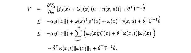 We choose the corrective control term pi(x) and the update law for  which implies that The feedback control law (5.105) is discontinuous at ωi(x) = 0.As discussed in Section 5.4.3, the discontinuous sign functions can be smoothed by using the tanh(·) function:  where ε > 0 is a small design constant. Another issue that arises with adaptive bounding control is the possible parameter drift of the bounding estimate The adaptive bounding control method is also used in adaptive approximation based control in order to address the issue of having the trajectory leave the approximation region. This is illustrated in Chapters 6 and 7. |
 instead of the true bounding vector θ. One of the key questions has to do with the design of the adaptive law for generating
  . As we will see, this is achieved again by Lyapunov analysis.
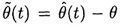 denote the parameter estimation error. Consider the augmented Lyapunov function
 as follows:
 . Therefore, both x(t) and
  remain bounded and x(t) converges to zero (using Barb lat's Lemma).
 . This may occur as a consequence of using the smooth approximation tahn(ωi(x)/ε), which may result in a small residual error. Moreover, in the presence of measurement noise or disturbances again the bounding parameter estimate
  may not converge. Since the right-hand side of (5.106) is nondecreasing, the presence of such residual errors (even if small) may cause the parameter drift of the estimate, which in turn will cause the feedback control signal to become large. This can be prevented by using a robust adaptive law, as described in Chapter 4. One of the available techniques is the dead-zone, which requires knowledge of the size of the residual error. Another method is the projection modification, which prevents the parameter estimate from becoming larger than a preselected level. Yet another approach is the σ modification.