In parallel with developments in adaptive nonlinear control, there has been a tremendous amount of activity in neural control and adaptive fuzzy approaches. In these studies, neural networks or fuzzy approximators are used to approximate unknown nonlinearities. The input/output response of the approximator is modified by adjusting the values of certain parameters, usually referred to as weights. From a mathematical control perspective, neural networks and fuzzy approximators represent just two classes of function approximators. Polynomials, splines, radial basis functions, and wavelets are examples of other function approximators that can be used and have been used in a similar setting. We refer to such approximation models with adaptivity features as adaptive approximators, and control methodologies that are based on them as adaptive approximation based control. Adaptive approximation based control encompasses a variety of methods that appear in the literature: intelligent control, neural control, adaptive fuzzy control, memory-based control, knowledge-based control, adaptive nonlinear control, and adaptive linear control. |
 During the last few years there have been significant developments in the control of highly uncertain, nonlinear dynamical systems. For systems with parametric uncertainty, adaptive nonlinear control has evolved as a powerful methodology leading to global stability and tracking results for a class of nonlinear systems. Advances in geometric nonlinear control theory, in conjunction with the development and refinement of new techniques, such as the backstepping procedure and tuning functions, have brought about the design of control systems with proven stability properties. In addition, there has been a lot of research activity on robust nonlinear control design methods, such as sliding mode control, Lyapunov redesign method, nonlinear damping, and adaptive bounding control. These techniques are based on the assumption that the uncertainty in the nonlinear functions is within some known, or partially known, bounding functions.
Chapter 5.1.2 - Linearizing Around a Trajectory
Consider the nonlinear system (5.1), where in this case the control objective is to design a control law such that the state x(t) tracks a desired vector signal xd (t). Let the tracking error be denoted by e(t) = x(t) xd (t). If a tracking controller is designed based on a linearization valid at some operating point xe ∈ The tracking objective is in general more suitably addressed by a control law that is designed based on linearization about the desired trajectory xd (t). Obviously, linearization around xd (t) assumes that this signal is available a priori. If xd (t) is not available but needs to be generated online possibly by an outer-loop controller, then small-signal linearization can be performed around a nominal trajectory x*(t), which is available a priori. Associated with a nominal trajectory x*(t) is a nominal control signal u*(t) and initial conditions Let  Using the Taylor series expansion of where F represents the higher-order terms of the Taylor series expansion. Since F contains the higher-order terms, it satisfies  In other words, as  In a linear approximation the higher-order terms are ignored. Hence, the small-signal linearization of (5.1) around the nominal trajectory x*(t) is given by  where z is the state of the linear model and the matrices A(t) : [0, ∞) 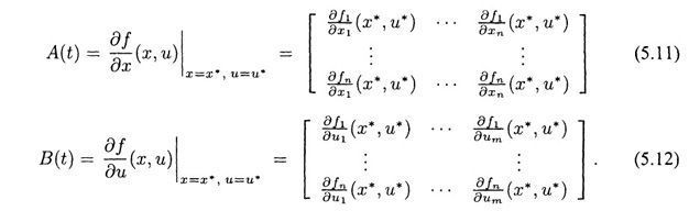 Now, suppose we select the control law as  If the pair (A(t), B(t)) is uniformly completely controllable, then there exists K(t) such that the closed-loop system (5.13) is asymptotically stable; therefore, z(t) → 0, which implies that x(t) → x*(t). If the nominal trajectory x*(t) coincides with the desired vector signal xd (t), then we achieve asymptotic convergence of the tracking error to zero. Clearly, the above stability arguments were based on the linear model. Applying the same control law to the nonlinear system we have  which implies  Again, linearizing the closed-loop system around x = x* = xd, u = u* yields  Therefore, applying the linear control law to the nonlinear system yields a locally asymptotically stable closed-loop system. In this case, locality is defined relative to the nominal trajectory (i.e., x(t) – x*(t)sufficiently small for all t > 0). If the nonlinear system has an output function then, again, we can proceed to obtain the C(t) and D(t) matrices. Linearization of the nonlinear system (5.5)-(5.6) around a nominal trajectory x*(t) produces a linear model of the form
where A(t), B(t) are given by (5.11)-(5.12), while C(t) ∈
Therefore, we see that linearizing around a trajectory yields similar results as linearizing around an equilibrium point, with the key difference that in the former case the linear model is time-varying. Next we present an example of linearizing around a nominal trajectory to illustrate the concepts introduced in this subsection. ■ EXAMPLE 5.2 A simple model of a satellite of unit mass moving in a plane can be described by the following equations of motion in polar coordinates [225]:
where, as shown in Figure 5.2, r(t) is the radius from the origin to the mass, θ(t) is the angle from a reference axis, u1(t) is the thrust force applied in the radial direction, u2(t) is the thrust force applied in the tangential direction, and Β is a constant parameter. With zero thrust forces (i.e., u1(t) = 0 and u2(t) = 0), the resulting solution can take various forms (ellipses, parabolas, or hyperbolas) depending on the initial conditions. In this example, we consider a simple circular trajectory with constant angular velocity (i.e., r(t) and To construct the state equation representation, let  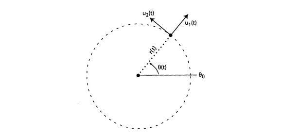 Figure 5.2: Point mass satellite moving in a planar gravitational orbit. The nominal trajectory is described by 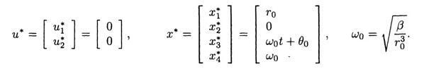 If we define 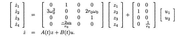
|
 n, then as xd (t) moves away from the equilibrium point, the state x(t) will try to follow it. However, as the distance between x(t) and xeincreases, the linear approximation may become increasingly inaccurate. As the accuracy of the linear approximation decreases, the designed linear controller may become unsuitable, thus possibly forcing x(t) even further away from the equilibrium xe.
 and
and  become small, F goes to zero faster than
  Using the Taylor series expansion, (5.10) can be rewritten
 . The closed-loop dynamics for the linear system are given by


 are both constant). It is easy to verify that with zero thrusts forces and the initial conditions
 the resulting nominal trajectory is r*(t) = r0 and θ*(t) = w0t + θ0. The objective is to linearize the model around this nominal trajectory.

 The equations of motion in the state coordinates are given by
 , then the small-signal linearized system (around the nominal trajectory) is given by