In parallel with developments in adaptive nonlinear control, there has been a tremendous amount of activity in neural control and adaptive fuzzy approaches. In these studies, neural networks or fuzzy approximators are used to approximate unknown nonlinearities. The input/output response of the approximator is modified by adjusting the values of certain parameters, usually referred to as weights. From a mathematical control perspective, neural networks and fuzzy approximators represent just two classes of function approximators. Polynomials, splines, radial basis functions, and wavelets are examples of other function approximators that can be used and have been used in a similar setting. We refer to such approximation models with adaptivity features as adaptive approximators, and control methodologies that are based on them as adaptive approximation based control. Adaptive approximation based control encompasses a variety of methods that appear in the literature: intelligent control, neural control, adaptive fuzzy control, memory-based control, knowledge-based control, adaptive nonlinear control, and adaptive linear control. |
 During the last few years there have been significant developments in the control of highly uncertain, nonlinear dynamical systems. For systems with parametric uncertainty, adaptive nonlinear control has evolved as a powerful methodology leading to global stability and tracking results for a class of nonlinear systems. Advances in geometric nonlinear control theory, in conjunction with the development and refinement of new techniques, such as the backstepping procedure and tuning functions, have brought about the design of control systems with proven stability properties. In addition, there has been a lot of research activity on robust nonlinear control design methods, such as sliding mode control, Lyapunov redesign method, nonlinear damping, and adaptive bounding control. These techniques are based on the assumption that the uncertainty in the nonlinear functions is within some known, or partially known, bounding functions.
Chapter 5.3.3 - Command Filtering Formulation
Much of the complexity that arises in the backstepping control laws that result from recursive application of Lemma 5.3.1 is due to the computation of the time derivative of the virtual control variables Consider the second-order syste
where x = [x1x2]T ∈
where x2cwill be defined by the backstepping controller. Let  be a smooth feedback control and define the smooth positive definite function  where To solve the tracking control problem for the system of eqns. (5.65)-(5.66) we use the following procedure:

Figure 5.4 displays a block diagram implementation of the above procedure. Note that Given the above procedure, we now analyze the stability of the control law. The tracking error dynamics can be written as 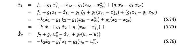  As defined in (5.70) and (5.73), the variables 1, 2 represent the filtered effect of the errors  Consider the following Lyapunov function candidate 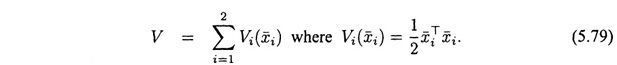 The time derivative of V along the solution of (5.77)-(5.78) is 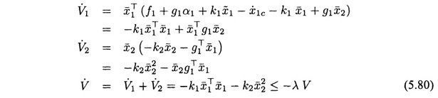 where λ = 2min(k1, k2) > 0. The fact that Lemma 5.3.2 Let the control law α1 solve the tracking problem for system  with Lyapunov function V1 satisfying (5.68). Then the controller of (5.69)-(5.73) solves the tracking problem (i.e., guarantees that x1(t) converges to yd (t)) for the system described by (5.65)-(5.66). Note that this lemma can be applied recursively n – 1 times to address a system with n states. An example of this will be presented below. Note that the result guarantees desirable properties for the compensated tracking errors
with input
The magnitude of the portion of the input defined by ( The goal of the derivation of this theorem was to avoid tedious algebraic manipulations involved in the computation of the backstepping control signal. Avoiding such computations will become increasingly important in backstepping approaches that include parameter adaptation. In the following example, we return to the problem of Example 5.7 using Lemma 5.3.2. ■ EXAMPLE 5.8 From (5.61)-(5.63) and (5.69), we have that
where
and for i = 1, 2, 3 we have This example should be compared with Example 5.7. For an n-th order system, standard backstepping will require as controller inputs |
 . The computation of these time derivatives becomes even more complex in applications where the functions ƒ and g are approximated online. This section presents an alternative formulation of the backstepping approach that decreases the algebraic complexity of the backstepping control law from that of eqn. (5.54).
 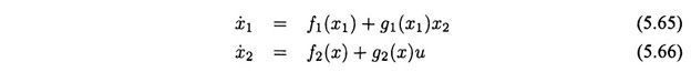 m
m 2 is the state, x2 ∈
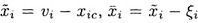
  , both of which lie in a region D for t ≥ 0 and both signals are assumed known. Define the tracking errors

 such that
 is positive definite in
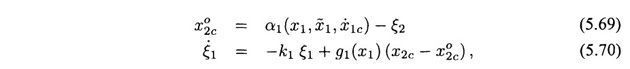
 is filtered to produce the command signal x2cand its derivative
  Such a filter is defined in Appendix A.4. Note that by the design of this command filter, the signal
  is bounded and small. Therefore, as long as g1(x1) is bounded, then ξ1 is bounded because it is the output of a stable linear filter with a bounded input.

 is filtered to produce
  is the control signal applied to the actual system. By the design of the command filter, the signal
  is bounded and small; therefore, if g2(x) is bounded, then ξ2 is the bounded output of a stable linear filter with a bounded input. If
 .
. is computed using
  , not
, not  is not used in the control law. It is not directly available and is tedious to compute for higher order systems.
 and
and  , respectively. The variables
  shows that the origin of the
  system is exponentially stable. Therefore, we can summarize these results in the following theorem.
 not the actual tracking errors
  . The difference between these two quantities is ξi, which is the output of the stable linear filter


 . Each pair
  and
and  is the output of second-order, low-pass, unity-gain filter of Figure A.4 with input
  , respectively. If
  is used as the control signal, then
 and ξ3 = 0.
  for i = 0, ... , n and will analytically compute
  . The command filtered approach will require as controller inputs only
  and will analytically compute only αi. The tradeoff is that the command filtered approach will require n scalar filters for the ξ variables and n command filters.