In parallel with developments in adaptive nonlinear control, there has been a tremendous amount of activity in neural control and adaptive fuzzy approaches. In these studies, neural networks or fuzzy approximators are used to approximate unknown nonlinearities. The input/output response of the approximator is modified by adjusting the values of certain parameters, usually referred to as weights. From a mathematical control perspective, neural networks and fuzzy approximators represent just two classes of function approximators. Polynomials, splines, radial basis functions, and wavelets are examples of other function approximators that can be used and have been used in a similar setting. We refer to such approximation models with adaptivity features as adaptive approximators, and control methodologies that are based on them as adaptive approximation based control. Adaptive approximation based control encompasses a variety of methods that appear in the literature: intelligent control, neural control, adaptive fuzzy control, memory-based control, knowledge-based control, adaptive nonlinear control, and adaptive linear control. |
 During the last few years there have been significant developments in the control of highly uncertain, nonlinear dynamical systems. For systems with parametric uncertainty, adaptive nonlinear control has evolved as a powerful methodology leading to global stability and tracking results for a class of nonlinear systems. Advances in geometric nonlinear control theory, in conjunction with the development and refinement of new techniques, such as the backstepping procedure and tuning functions, have brought about the design of control systems with proven stability properties. In addition, there has been a lot of research activity on robust nonlinear control design methods, such as sliding mode control, Lyapunov redesign method, nonlinear damping, and adaptive bounding control. These techniques are based on the assumption that the uncertainty in the nonlinear functions is within some known, or partially known, bounding functions.
Chapter 5.3.2 - Higher Order Systems
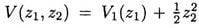
Consider the system model 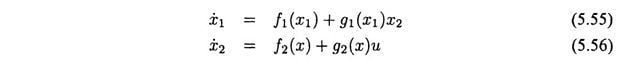 where  where W1(z1) is a positive definite function. Our objective is to define u such that the system of equations (5.55)-(5.56) will have x1 tracking yd(i.e., z1 convergent to zero). We define z2 = x2–α. Then the (z1, z2) dynamics are described by
where
Consider 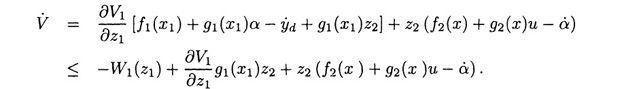 Therefore, if g2(x) ≠ 0 and the control signal u is selected as  with k2 > 0 being a design parameter, then we have  which is negative definite. Therefore, we have proven Lemma 5.3.1. Note that this lemma can be applied recursively to achieve tracking control for higher order systems. Lemma 5.3.1 Given a system in the form of (5.55)-(5.56) and known functions ■ EXAMPLE 5.7 Consider the third-order system 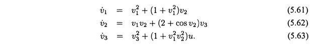 The tracking control design problem is solved in three steps, where the second and third steps will utilize Lemma 5.3.1. Step 1. In this step, we find a control signal α1 to solve the tracking control problem for the system
If we select
where z1 = v1–yd and k1 > 0, the controlled z1 dynamics are
and the time derivative of
where Step 2. We are now in a position to use Lemma 5.3.1 to specify a control signal α2 to solve the tracking problem for the second order subsystem  To utilize the lemma, we let x1 = v1, x2 = v2,
where k2 is a positive design parameter. The Lyapunov function for the second order tracking error dynamics would be
Where Step 3. Now, we are in a position to use Lemma 5.3.1 to specify a control signal u to solve the original three state tracking problem To utilize the lemma, we let    where k3 is a positive design parameter. As a result of the lemma, the control law given by (5.64) results in globally exponentially stable tracking error dynamics.
|
 Define z1 = x1 – ydwhere yd (t) is the signal vector to be tracked. For this system, we assume that we know scalar virtual control functions
  and positive definite V1(z1) such that
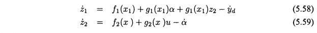
 . The time derivative of V along the solutions of (5.58)-(5.59) is given by
 and positive definite V1(z1) satisfying (5.57), then for u specified according to (5.60), the tracking error dynamics of (5.58)-(5.59) are asymptotically stable. If V1 is radially unbounded and all assumptions hold globally, then the tracking error dynamics are globally asymptotically stable.
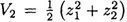 , which has a time derivative satisfying
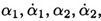 and finally u. These computations will involve
  In general, the computation of the quantities
  can be algebraically tedious, especially for systems of order larger than two or three.