Sliding mode control is a methodology based on the principle that it is easier to control a first-order system than a n-th order system. Therefore, this approach can be viewed as a way to reduce a higher-order control problem into a simpler one for which there are known feedback control methods. This simplification comes at the expense of using a large control effort, which, as discussed earlier in the chapter, could be the source of other potential problems, especially in the presence of measurement noise or high frequency unmodeled dynamics. The sliding mode control methodology can be applied to several classes of nonlinear systems. Here, we consider its application to a class of feedback linearizable systems.

Consider an n-th order nonlinear system of the form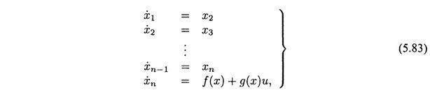

where it is assumed that ƒ and g are unknown and g(x) ≥ g₀ > 0 for all x ∈ ⁿ. The control objective is for y(t) = x₁(t) to track a desired signal y_d (t). Let e = y – y_d be the tracking error. The sliding mode surface s is defined as

where the coefficients {λ₁, λ₂, ... λ_{n - 1}} are selected such that the characteristic polynomial (in p)

is Hurwitz (i.e., all the roots of the polynomial are in the left-half complex plane). The manifold described by s – 0 is referred to as the sliding manifold or sliding surface and has dimension (n - 1). The objective of sliding mode control is to steer the trajectory onto this sliding manifold. This is achieved by forcing the variable s to zero in finite time. By design of the sliding surface, if x is on the sliding surface defined by s = 0, then

Since the polynomial given by (5.85) is Hurwitz, once on the sliding manifold the tracking error will go to zero with a transient behavior characterized by the selected coefficients {λ₁, λ₂, ... λ_{n - 1}} (i.e., exponentially fast).

The sliding mode control objective can be achieved if the control law u is chosen such that

where k > 0. In this case, the upper right-hand derivative of s(t) satisfies the differential inequality

which implies that the trajectory reaches the manifold 5 = 0 in finite time.

Following (5.84), the derivative of s(t) satisfies

If ƒ and g were known function, then we could choose the control law

where k > 0 is a design variable and sgn(·) denotes the sign function:

Based on this control law, the derivative of s(t) satisfies

which implies

Now consider the case where ƒ and g are unknown but the designer has a known upper bound (x, t) such that

Suppose that the control law is selected as

where ₀ > 0 is a design constant. Now, let

be the Lyapunov function candidate. The derivative of V is given by

where g₀ is defined in (5.83). Therefore, we have achieved the desired objective of forcing the trajectory onto the sliding manifold in finite time. It is interesting to note that this is achieved without specific knowledge of ƒ and g, just the upper bound (x, t).

Despite the resulting stability and convergence properties of the sliding mode control approach, it has two key drawbacks in its standard form. The sliding mode control law given by (5.86) has two components, the gain n(x, t) + n₀ and the switching function sgn(s), both of which can create problems:

• (High-Gain) Note that the gain term is the result of taking an upper bound on the uncertainty. In general, this creates a high-gain feedback control, which can create problems in the presence of measurement noise and high-frequency unmodeled dynamics. Moreover, high-gain feedback may require significant control effort, which can be expensive and/or may cause saturation of the actuators. In practice, high-gain feedback control is to be avoided.
  
  
• (Chattering) The switching function sgn(s) causes the control gain to switch from (x, t) + ₀ to – ( (x, t) + ₀) every time the trajectory crosses the sliding manifold. Although in theory the trajectory is suppose to "slide" on the sliding manifold, in
  
  
  

Figure 5.5: Graphical illustration of sliding mode control and chattering as a result of imperfection in the switching.

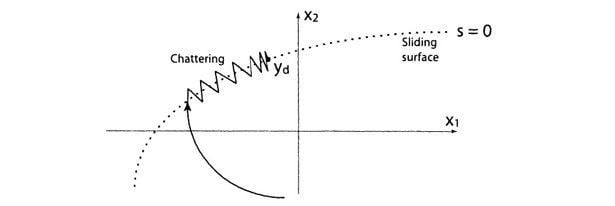
practice there are imperfections and delays in the witching devices, which lead to chattering. This is illustrated in Figure 5.5. Chattering causes significant problems in the feedback control system, especially if it is associated with high gains. For example, chattering may excite high-frequency dynamics which were neglected in the design model, it can cause wear and tear of moving mechanical parts and it can cause high heat losses in electrical power systems.

Research in sliding mode control has developed some techniques for addressing the above two issues. The high gain problem can be reduced by using as much a priori information as possible, thus canceling the known nonlinearities and employing an upper bound only for the unknown portions of the nonlinearities. The chattering problem can also be addressed, partially, by employing a continuous approximation of the sign function. The tradeoff in the use of this approximation is that only uniform boundedness of solutions can be proved. Despite these remedies, the sliding mode methodology is based on the principle of bounding the uncertainty by a larger function, and as a result it is a conservative control approach. In this text, we present a methodology for "learning" or approximating the uncertainty online, instead of using an upper bound for it. However, the approximation will be valid only within a certain compact region D. In order to achieve stability outside this region, we will rely on bounding control techniques such as sliding mode.