In parallel with developments in adaptive nonlinear control, there has been a tremendous amount of activity in neural control and adaptive fuzzy approaches. In these studies, neural networks or fuzzy approximators are used to approximate unknown nonlinearities. The input/output response of the approximator is modified by adjusting the values of certain parameters, usually referred to as weights. From a mathematical control perspective, neural networks and fuzzy approximators represent just two classes of function approximators. Polynomials, splines, radial basis functions, and wavelets are examples of other function approximators that can be used and have been used in a similar setting. We refer to such approximation models with adaptivity features as adaptive approximators, and control methodologies that are based on them as adaptive approximation based control. Adaptive approximation based control encompasses a variety of methods that appear in the literature: intelligent control, neural control, adaptive fuzzy control, memory-based control, knowledge-based control, adaptive nonlinear control, and adaptive linear control. |
 During the last few years there have been significant developments in the control of highly uncertain, nonlinear dynamical systems. For systems with parametric uncertainty, adaptive nonlinear control has evolved as a powerful methodology leading to global stability and tracking results for a class of nonlinear systems. Advances in geometric nonlinear control theory, in conjunction with the development and refinement of new techniques, such as the backstepping procedure and tuning functions, have brought about the design of control systems with proven stability properties. In addition, there has been a lot of research activity on robust nonlinear control design methods, such as sliding mode control, Lyapunov redesign method, nonlinear damping, and adaptive bounding control. These techniques are based on the assumption that the uncertainty in the nonlinear functions is within some known, or partially known, bounding functions.
Chapter 5.2.1 - Scalar Input-State Linearization
To illustrate the main intuitive idea behind feedback linearization, we start by considering the simple scalar system
where u is the control input, y is the measured output, and the nonlinear functions ƒ, g are assumed to be known a priori. The control objective is to design a control law that generates u such that u(t) and y(t) remain bounded and y(t) tracks a desired function yd (t). We will assume throughout that yd (t) and all of its derivatives that are required for computing the control signal are in fact available, continuous, and bounded. Section A.4 of the appendix discusses prefiltering, which is one method to ensure the validity of this assumption. For this scalar system it is straightforward to see that, assuming that g(y) ≠ 0, the control law  where am > 0 is a design constant, achieves the control objective. Specifically, with the above feedback control algorithm, the tracking error e(t) = y(t) – yd(t) satisfies A key observation for the reader is that implementation of the feedback control algorithm (5.14) is feasible in all scenarios of desired trajectories ydonly if the function g(y) ≠ 0 for all y ∈ ■ EXAMPLE 5.3 It is important to note that even if g(y) = 0 at a crucial part of the state-space, that does not necessarily imply that the system is uncontrollable. For example, consider the input-output system
The control law (5.14) illustrates the use of the controller for canceling nonlinearities. Specifically, as we can see from (5.14), the nonlinearities ƒ and g in the open-loop system are cancelled by the controller. This converts the system into one with linear error dynamics, for which there are known control design and analysis methods. In fact, (5.14), can be rewritten as  where (5.15) is a feedback linearizing operator that causes the closed-loop system to transform to the linear system
These comments also apply to feedback linearization when it is applied to higher order systems. Appended Integrators. One role of integrators in control laws is to force the tracking error to zero in the presence of model error, disturbances, and input type. The required number of integrators as a function of the type of the input to be tracked is discussed in most text books on control system design, e.g., [66, 86, 140]. Integrators can have similar utility in nonlinear control applications. Integrators can be included in the control law and control design analysis by various approaches such as that discussed in Exercise 1.3 and the following. In addition to the tracking error e(t) = y(t) – yd (t) define  where c > 0. It is noted that eF (t) is a linear combination of the tracking error and the integral of the tracking error that can be thought of as providing a PI controller (proportional-integral control). For implementation and analysis, the system state space model will include one appended controller state to compute the integral of the tracking error. From (5.17), we obtain  (see also (6.35)). This control law results in |

 Hence, the tracking error converges to zero exponentially fast from any initial condition (global stability results).
 . Otherwise, if g(y) approaches zero then the control effort becomes large, causing saturation of the control input and possibly leading to instability. This problem, which arises due to the lack of controllability at some values of the state-space, is referred to as the stabilizability problem.
 and (5.16) is a linear stabilizing controller for the linearized tracking problem. Many other linear controllers could be selected. Even for this simple system we can extract some key observations:
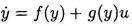 over the domain of validity of that model. There are no approximations. This is distinct from the small signal linearization of Section 5.1, which was exact only at a single point.
 . Therefore, from a theoretical perspective, the reference input tracking bandwidth of this controller is infinite. In fact, this bandwidth will be limited by physical constraints, such as the actuators, and must be accounted for in the design of the system that generates ydand its derivatives.
 ; hence, to force eF (t) to zero, the control law (5.15) is modified to
 . It is easy to see that if eF (t) converges to zero then so does e(t) (notice that
  ).
).