D.1 Sinusoidal Steady-State Response

Analysis of the sinusoidal steady-state response of digital filters will lead to the development of the magnitude and phase responses of digital filters. Let us look at the following digital filter with a digital transfer function H( z) and a complex sinusoidal input

(D.1)

where ? = ?T is the normalized digital frequency, while T is the sampling period and y( n) denotes the digital output, as shown in Figure D.1.

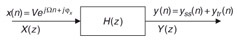Figure D.1: Steady-state response of the digital filter.

The z-transform output from the digital filter is then given by

(D.2)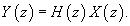

Since X( z) = , we have

(D.3)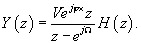

Based on the partial fraction expansion, Y( z)/ z can be expanded as the following form:

(D.4)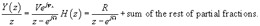

Multiplying the factor ( z = e ^j?) on both sides of Equation (D.4) yields

(D.5)

Substituting z = e ^j?, we get the residue as

Then substituting R = Ve ^j? H(e ^j?) back into Equation (D.4) results in

(D.6)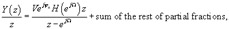

and multiplying z on both sides of Equation (D.6) leads to

(D.7)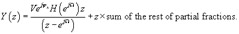

Taking the inverse z-transform leads to two parts of the solution:

(D.8)

From Equation (D.8), we have the steady-state response

(D.9)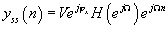

and the transient response

(D.10)

Note that since the digital filter is a stable system, and the locations of its poles must be inside the unit circle on the z-plane, the transient response will be settled...